Intro to the tidyverse

The intent of this chapter is to get you familiarized with the process of going from data import to visualization. This section will walk you through the core concepts in the packages dplyr and ggplot2, which are parts of the tidyverse. The tidyverse is a collection of R packages developed by RStudio’s chief scientist Hadley Wickham. These packages work well together as part of larger data analysis pipeline. You will gain a tremendous level of experience and repetitions with these packages, which will solidify your knowledge. The later chapters will solidify your understanding of all concepts in this part.
Theory Input
Packages
You know what functions are and how to write your own functions. You’re not the only person writing your own functions with R. Many people design tools that can help people analyze data. They provide those functions and objects for free in wrapped up packages. You only have to download and install them. Each R package is hosted at http://cran.r-project.org, the same website that hosts R (often interesting new R packages are only available on GitHub, because submitting to CRAN is a lot more work than just providing a version on github). However, you don’t need to visit the website (or github) to download an R package. You can download packages straight from R’s command line.
Video instructions to install R packages
These are the basic commands you will need for installing and loading packages in your current R session:
# install package from CRAN
install.packages("packagename")

# load the package to use in the current R session
library("packagename")

# use a particular function within a package without loading the package
packagename::function_name()Downlaod the following file and place in your getting_started folder. Try running the commands to install some of the packages we are going to use throughout this class.
Windows Users: You will get a warning if Rtools is not installed. See the last session for install instructions.
If you get a message saying “Do you want to install from source the packages which need compilation?", selecting “No” will revert to the latest compiled version which may not be the most recent on CRAN (the respository that people and organizations store open source packages on). Selecting “Yes” will download the latest, and use your machine to do the compiling. This may take longer.
If you get errors do the following:
- Try installing one package at a time. Find which package has the error and isolate it. Then proceed to step 2.
- Restart R by exiting RStudio and reopening. Retry installing the problem package. If this does not work, proceed to step 3.
- Google “R” + “install.packages” + the error message. Chances are 99% likely that someone else has experienced an error like yours.
If otherwise unsuccessful, contact me and I will do my best to troubleshoot.
Pipes
%>% throughout this class. The “pipe” is from the magrittr package (included in the tidyverse). The point of the pipe is to help you write code in a way that is easier to read and understand. It makes your code more readable by structuring sequences of data operations left-to-right (as opposed to from the inside and out). The pipe makes your code read more like a sentence, branching from left to right. You can read it as a series of imperative statements: group, then summarise, then filter. As suggested by this reading, a good way to pronounce %>% when reading code is “then”. Mathematically it can be expressed like the following:x %>% fis equivalent tof(x)x %>% f(y)is equivalent tof(x, y)x %>% f %>% g %>% his equivalent toh(g(f(x)))
Instead of writing this:
data <- iris
data <- head(data, n=3)
you can write the code like this:
# The easiest way to get magrittr is to load the whole tidyverse:
library("tidyverse")
# Alternatively, load just magrittr:
library("magrittr")

iris %>% head(n=3)
When coupling several function calls with the pipe-operator, the benefit will become more apparent. Consider this pseudo example:
the_data <-
  read.csv('/path/to/data/file.csv') %>%
  subset(variable_a > x) %>%
  transform(variable_c = variable_a/variable_b) %>%
  head(100)
Tibbles
tibbles instead of R’s traditional data.frame. Tibbles are data frames, but they tweak some older behaviours to make life a little easier. R is an old language, and some things that were useful 10 or 20 years ago now get in your way. In most places, the term tibble and data frame will be used interchangeably.- tibble is one of the unifying features of tidyverse,
- it is a better data.frame realization,
- objects of the class data.frame can be coerced to tibble using
as_tibble()
When you print a tibble, the output shows:
- all columns that fit the screen
- first 10 rows
- data type for each column
A tibble is being constucted like this:
tibble(
    x = 1:50,
    y = runif(50),
    z = x + y^2,
    outcome = rnorm(50)
  )
Check yourself how dataframes and tibbles print differently (you can use for an example the built in dataframe cars):
class(cars)
## "data.frame"

cars_tbl <- as_tibble(cars)
class(cars_tbl)
## "tbl_df"     "tbl"        "data.frame"
There are multiple ways of subsetting (retrieving just parts of the date) tibbles:
# This way applies to dataframes and tibbles
vehicles <- as_tibble(cars[1:5,])
vehicles[['speed']]
vehicles[[1]]
vehicles$speed

# Using placeholders with the pipe
vehicles %>% .$dist
vehicles %>% .[['dist']]
vehicles %>% .[[2]]
Import
Before you can manipulate data with R, you need to import the data into R’s memory, or build a connection to the data that R can use to access the data remotely.
How you import your data will depend on the format of the data. The most common way to store small data sets is as a plain text file. Data may also be stored in a proprietary format associated with a specific piece of software, such as SAS, SPSS, or Microsoft Excel. Data used on the internet is often stored as a JSON or XML file. Large data sets may be stored in a database or a distributed storage system.
When you import data into R, R stores the data in your computer’s RAM while you manipulate it. This creates a size limitation: truly big data sets should be stored outside of R in a database or distributed storage system. You can then create a connection to the system that R can use to access the data without bringing the data into your computer’s RAM.
The tidyverse offers the following packages for importing data:
readrfor reading flat files like .csv filesreadxlfor .xls and .xlsx sheets.havenfor SPSS, Stata, and SAS data.googledriveto interact with files on Google Drive from R.
There are a handful of other packages that are not in the tidyverse, but are tidyverse-adjacent. They are very useful for importing data from other sources (we will use them in the next session):
- jsonlite for JSON.
- xml2 for XML.
- httr for web APIs.
- rvest for web scraping.
- DBI for relational databases. To connect to a specific database, you’ll need to pair DBI with a specific backend like RSQLite, RPostgres, or odbc. Learn more at https://db.rstudio.com.
Example
# Loading data (can also be achieved by clicking on "Import Dataset > From Text (readr)" in the upper right corner)
library(readr)
dataset_tbl <- read_csv("data.csv")
# In case of possible parsing errors, analyze them with problems()
readr::problems(dataset_tbl)

# Writing data
write_csv(dataset_tbl, "data.csv")

# Saving in csv (or tsv) does mean you loose information about the type of data in particular columns. You can avoid this by using  write_rds() and read_rds() to read/write objects in R binary rds format.
write_rds(dataset_tbl, "data.rds")
Tidy
Reshaping your data with tidyr
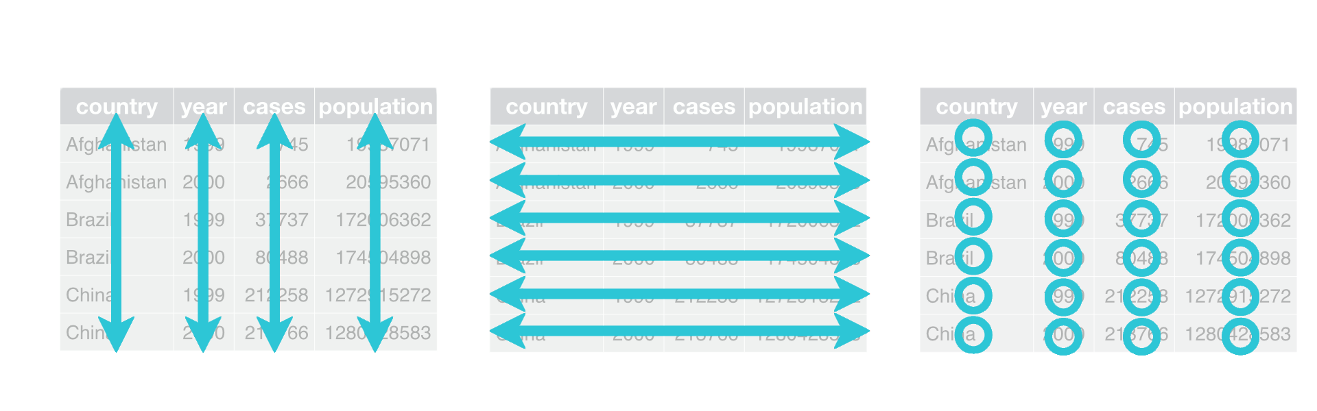
The Concept of Tidy Data
- each and every observation is represented as exactly one row,
- each and every variable is represented by exactly one column,
- thus each data table cell contains only one value.
Usually data are untidy in only one way. However, if you are unlucky, they are really untidy and thus a pain to work with…
Exercise
Which of these data are tidy?
| Sepal.Length | Sepal.Width | Petal.Length | Petal.Width | Species |
|---|---|---|---|---|
| 5.1 | 3.5 | 1.4 | 0.2 | setosa |
| 4.9 | 3.0 | 1.4 | 0.2 | setosa |
| 4.7 | 3.2 | 1.3 | 0.2 | setosa |
| Species | variable | value |
|---|---|---|
| setosa | Sepal.Length | 5.1 |
| setosa | Sepal.Length | 4.9 |
| setosa | Sepal.Length | 4.7 |
| Sepal.Length | 5.1 | 4.9 | 4.7 | 4.6 |
|---|---|---|---|---|
| Sepal.Width | 3.5 | 3.0 | 3.2 | 3.1 |
| Petal.Length | 1.4 | 1.4 | 1.3 | 1.5 |
| Petal.Width | 0.2 | 0.2 | 0.2 | 0.2 |
| Species | setosa | setosa | setosa | setosa |
| Sepal.L.W | Petal.L.W | Species |
|---|---|---|
| 5.1/3.5 | 1.4/0.2 | setosa |
| 4.9/3 | 1.4/0.2 | setosa |
| 4.7/3.2 | 1.3/0.2 | setosa |
| --- | --- | --- |
Solution
To illustrate how we can make data tidy easily, we are using modified variants of the diamonds dataset from the ggplot2 package. Try to make the data tidy by looking at the corresponding help pages of each provided function.
- Tidying data with
pivot_longer(): Use, if some of your column names are actually values of a variable. Alternatively you can usegather(), but it is recommended to usepivot_longer(), because the other function is no longer being maintained.
library(tidyverse)
diamonds2 <- readRDS("diamonds2.rds")

diamonds2 %>% head(n = 5)
## # A tibble: 5 x 3
##   cut     `2008` `2009`
##   <chr>    <dbl>  <dbl>
## 1 Ideal      326    332
## 2 Premium    326    332
## 3 Good       237    333
## 4 Premium    334    340
## 5 Good       335    341
Solution
diamonds2 %>%
pivot_longer(cols = c("2008", "2009"),
names_to = 'year',
values_to = 'price') %>%
head(n = 5)
## # A tibble: 5 x 3
## cut year price
## <chr> <chr> <dbl>
## 1 Ideal 2008 326
## 2 Ideal 2009 332
## 3 Premium 2008 326
## 4 Premium 2009 332
## 5 Good 2008 237The wide (original) format might be good for business reports, but it is not good for doing analyses. If we wanted to predict the price based on the other data (with a simple linear regression), we need the long format:
model <- lm(price ~ ., data = diamonds2_long)
model
## Call:
## lm(formula = price ~ ., data = diamonds2_long)
## Coefficients:
## (Intercept) cutIdeal cutPremium year2009
## 237 89 89 6- Tidying data with
pivot_wider(): Use, if some of your observations are scattered across many rows. Alternatively you can usespread(), but it is recommended to usepivot_wider(), because the other function is no longer being maintained.
diamonds3 <- readRDS("diamonds3.rds")

diamonds3 %>% head(n = 5)
## # A tibble: 5 x 5
##   cut     price clarity dimension measurement
##   <ord>   <dbl> <ord>   <chr>           <dbl>
## 1 Ideal     326 SI2     x                3.95
## 2 Premium   326 SI1     x                3.89
## 3 Good      327 VS1     x                4.05
## 4 Ideal     326 SI2     y                3.98
## 5 Premium   326 SI1     y                3.84
Solution
diamonds3 %>%
pivot_wider(names_from = "dimension",
values_from = "measurement") %>%
head(n = 5)
## # A tibble: 3 x 6
## cut price clarity x y z
## <ord> <dbl> <ord> <dbl> <dbl> <dbl>
## 1 Ideal 326 SI2 3.95 3.98 2.43
## 2 Premium 326 SI1 3.89 3.84 2.31
## 3 Good 327 VS1 4.05 4.07 2.31- Tidying data with
separate(): If some of your columns contain more than one value, use separate:
diamonds4 <- readRDS("diamonds4.rds")

diamonds4
## # A tibble: 5 x 4
##   cut     price clarity dim
##   <ord>   <dbl> <ord>   <chr>
## 1 Ideal     326 SI2     3.95/3.98/2.43
## 2 Premium   326 SI1     3.89/3.84/2.31
## 3 Good      327 VS1     4.05/4.07/2.31
## 4 Premium   334 VS2     4.2/4.23/2.63
## 5 Good      335 SI2     4.34/4.35/2.75
Solution
diamonds4 %>%
separate(col = dim,
into = c("x", "y", "z"),
sep = "/",
convert = T)
## # A tibble: 5 x 6
## cut price clarity x y z
## <ord> <dbl> <ord> <dbl> <dbl> <dbl>
## 1 Ideal 326 SI2 3.95 3.98 2.43
## 2 Premium 326 SI1 3.89 3.84 2.31
## 3 Good 327 VS1 4.05 4.07 2.31
## 4 Premium 334 VS2 4.2 4.23 2.63
## 5 Good 335 SI2 4.34 4.35 2.75- Tidying data with
unite(): use to paste together multiple columns into one:
diamonds5 <- readRDS("diamonds5.rds")

diamonds5
## # A tibble: 5 x 7
##   cut     price clarity_prefix clarity_suffix     x     y     z
##   <ord>   <dbl> <chr>          <chr>          <dbl> <dbl> <dbl>
## 1 Ideal     326 SI             2               3.95  3.98  2.43
## 2 Premium   326 SI             1               3.89  3.84  2.31
## 3 Good      327 VS             1               4.05  4.07  2.31
## 4 Premium   334 VS             2               4.2   4.23  2.63
## 5 Good      335 SI             2               4.34  4.35  2.75
Solution
diamonds5 %>%
unite(clarity, clarity_prefix, clarity_suffix, sep = '')
## # A tibble: 5 x 6
## cut price clarity x y z
## <ord> <dbl> <ord> <dbl> <dbl> <dbl>
## 1 Ideal 326 SI2 3.95 3.98 2.43
## 2 Premium 326 SI1 3.89 3.84 2.31
## 3 Good 327 VS1 4.05 4.07 2.31
## 4 Premium 334 VS2 4.2 4.23 2.63
## 5 Good 335 SI2 4.34 4.35 2.75Transform
Often you’ll need to create some new variables or summaries, or maybe you just want to rename the variables or reorder the observations in order to make the data a little easier to work with. dplyr is a grammar of data manipulation, providing a consistent set of verbs that help you solve the most common data manipulation challenges. The following five key dplyr functions allow you to solve the vast majority of your data manipulation challenges:
filter()picks cases based on their values (formula based filtering). Useslice()for filtering with row numbers. So both can be used for selecting the relevant rows.
library(ggplot2) # To load the diamonds dataset
library(dplyr)
diamonds %>%
    filter(cut == 'Ideal' | cut == 'Premium', carat >= 0.23) %>%
    head(5)

## # A tibble: 5 x 10
##   carat cut     color clarity depth table price     x     y     z
##
## 1 0.23  Ideal   E     SI2      61.5    55   326  3.95  3.98  2.43
## 2 0.290 Premium I     VS2      62.4    58   334  4.2   4.23  2.63
## 3 0.23  Ideal   J     VS1      62.8    56   340  3.93  3.9   2.46
## 4 0.31  Ideal   J     SI2      62.2    54   344  4.35  4.37  2.71
## 5 0.32  Premium E     I1       60.9    58   345  4.38  4.42  2.68

diamonds %>%
   filter(cut == 'Ideal' | cut == 'Premium', carat >= 0.23) %>%
   slice(3:4)

## # A tibble: 2 x 10
##   carat cut   color clarity depth table price     x     y     z
##
## 1  0.23 Ideal J     VS1      62.8    56   340  3.93  3.9   2.46
## 2 0.31 Ideal J SI2 62.2 54 344 4.35 4.37 2.71 | Operator | Description |
|---|---|
| < | less than |
| <= | less than or equal to |
| > | greater than |
| >= | greater than or equal to |
| == | exactly equal to |
| != | not equal to |
| !x | Not x. Gives the opposite logical value. |
| x | y | x OR y |
| x & y | x AND y |
arrange()changes the ordering of the rows
diamonds %>%
  arrange(cut, carat, desc(price))

# A tibble: 53,940 x 10
   carat cut   color clarity depth table price     x     y     z

 1 0.22  Fair  E     VS2      65.1    61   337  3.87  3.78  2.49
 2 0.23  Fair  G     VVS2     61.4    66   369  3.87  3.91  2.39
 3 0.25  Fair  F     SI2      54.4    64  1013  4.3   4.23  2.32
 4 0.25  Fair  D     VS1      61.2    55   563  4.09  4.11  2.51
 5 0.25  Fair  E     VS1      55.2    64   361  4.21  4.23  2.33
 6 0.27  Fair  E     VS1      66.4    58   371  3.99  4.02  2.66
 7 0.290 Fair  F     SI1      55.8    60  1776  4.48  4.41  2.48
 8 0.290 Fair  D     VS2      64.7    62   592  4.14  4.11  2.67
 9 0.3   Fair  D     IF       60.5    57  1208  4.47  4.35  2.67
10 0.3   Fair  E     VVS2     51      67   945  4.67  4.62  2.37
# … with 53,930 more rows
The NAs always end up at the end of the rearranged tibble.
select()picks (or removes) variables based on their names
diamonds %>%
  select(color, clarity, x:z) %>%
  head(n = 5)

## # A tibble: 5 x 5
##   color clarity     x     y     z
##
## 1 E     SI2      3.95  3.98  2.43
## 2 E     SI1      3.89  3.84  2.31
## 3 E     VS1      4.05  4.07  2.31
## 4 I     VS2      4.2   4.23  2.63
## 5 J     SI2      4.34  4.35  2.75
Exclusive select:
diamonds %>%
  select(-(x:z)) %>%
  head(n = 5)

## # A tibble: 5 x 7
##   carat cut     color clarity depth table price
##
## 1 0.23  Ideal   E     SI2      61.5    55   326
## 2 0.21  Premium E     SI1      59.8    61   326
## 3 0.23  Good    E     VS1      56.9    65   327
## 4 0.290 Premium I     VS2      62.4    58   334
## 5 0.31  Good    J     SI2      63.3    58   335
Select helpers
starts_with()/ends_with(): helper that selects every column tht starts with a prefix or ends with a suffixcontains(): A select helper that selects any column containing a string of text.everything(): a select() helper that selects every column that has not already been selected. Good for reordering.
diamonds %>%
  select(x:z, everything()) %>%
  head(n = 5)

## # A tibble: 5 x 10
##       x     y     z carat cut     color clarity depth table price
##
## 1  3.95  3.98  2.43 0.23  Ideal   E     SI2      61.5    55   326
## 2  3.89  3.84  2.31 0.21  Premium E     SI1      59.8    61   326
## 3  4.05  4.07  2.31 0.23  Good    E     VS1      56.9    65   327
## 4  4.2   4.23  2.63 0.290 Premium I     VS2      62.4    58   334
## 5 4.34 4.35 2.75 0.31 Good J SI2 63.3 58 335 rename()changes the name of a column.
diamonds %>%
  rename(var_x = x) %>%
  head(n = 5)

## # A tibble: 5 x 10
##   carat cut     color clarity depth table price var_x     y     z
##
## 1 0.23  Ideal   E     SI2      61.5    55   326  3.95  3.98  2.43
## 2 0.21  Premium E     SI1      59.8    61   326  3.89  3.84  2.31
## 3 0.23  Good    E     VS1      56.9    65   327  4.05  4.07  2.31
## 4 0.290 Premium I     VS2      62.4    58   334  4.2   4.23  2.63
## 5 0.31 Good J SI2 63.3 58 335 4.34 4.35 2.75 mutate()adds new variables that are functions of existing variables and preserves existing ones.transmute()adds new variables and drops existing ones.
diamonds %>%
  mutate(p = x + z, q = p + y) %>%
  select(-(depth:price)) %>%
  head(n = 5)

## # A tibble: 5 x 9
##   carat cut     color clarity     x     y     z     p     q
##
## 1 0.23  Ideal   E     SI2      3.95  3.98  2.43  6.38  10.4
## 2 0.21  Premium E     SI1      3.89  3.84  2.31  6.2   10.0
## 3 0.23  Good    E     VS1      4.05  4.07  2.31  6.36  10.4
## 4 0.290 Premium I     VS2      4.2   4.23  2.63  6.83  11.1
## 5 0.31  Good    J     SI2      4.34  4.35  2.75  7.09  11.4
diamonds %>%
transmute(carat, cut, sum = x + y + z) %>%
head(n = 5)
## # A tibble: 5 x 3
## carat cut sum
##
## 1 0.23 Ideal 10.4
## 2 0.21 Premium 10.0
## 3 0.23 Good 10.4
## 4 0.290 Premium 11.1
## 5 0.31 Good 11.4 bind_cols()andbind_rows(): binds two tibbles column-wise or row-wise.group_by()andsummarize()reduces multiple values down to a single summary
diamonds %>%
  group_by(cut) %>%
  summarize(max_price  = max(price),
            mean_price = mean(price),
            min_price  = min(price))

## # A tibble: 5 x 4
##   cut       max_price mean_price min_price
##
## 1 Fair          18574      4359.       337
## 2 Good          18788      3929.       327
## 3 Very Good     18818      3982.       336
## 4 Premium       18823      4584.       326
## 5 Ideal 18806 3458. 326 glimpse()can be used to see the columns of the dataset and display some portion of the data with respect to each attribute that can fit on a single line. You can apply this function to get a glimpse of your dataset. It is similar to the base functionstr().
glimpse(diamonds)
## Rows: 53,940
## Columns: 10
## $ carat <dbl> 0.23, 0.21, 0.23, 0.29, 0.31, 0.24, 0.24, 0.26, 0.22, 0.23, …
## $ cut <ord> Ideal, Premium, Good, Premium, Good, Very Good, Very Good, …
## $ color <ord> E, E, E, I, J, J, I, H, E, H, J, J, F, J, E, E, I, J, J, J, …
## $ clarity <ord> SI2, SI1, VS1, VS2, SI2, VVS2, VVS1, SI1, VS2, VS1, SI1, VS1, …
## $ depth <dbl> 61.5, 59.8, 56.9, 62.4, 63.3, 62.8, 62.3, 61.9, 65.1, 59.4, …
## $ table <dbl> 55, 61, 65, 58, 58, 57, 57, 55, 61, 61, 55, 56, 61, 54, 62, …
## $ price <int> 326, 326, 327, 334, 335, 336, 336, 337, 337, 338, 339, 340, 3…
## $ x <dbl> 3.95, 3.89, 4.05, 4.20, 4.34, 3.94, 3.95, 4.07, 3.87, 4.00, …
## $ y <dbl> 3.98, 3.84, 4.07, 4.23, 4.35, 3.96, 3.98, 4.11, 3.78, 4.05, …
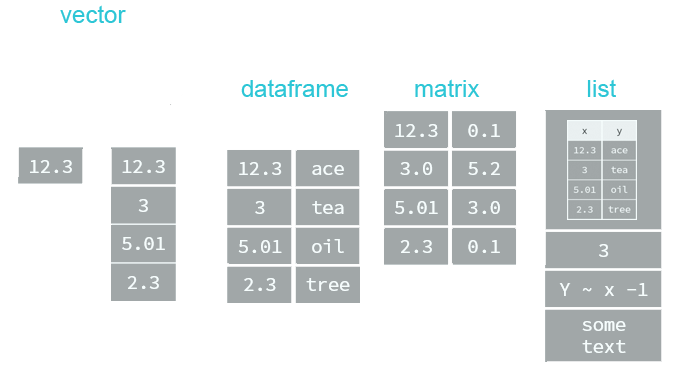
## $ z <dbl> 2.43, 2.31, 2.31, 2.63, 2.75, 2.48, 2.47, 2.53, 2.49, 2.39, …Data types and data structures
Everything in R is an object. R has 6 basic data types. U can use typeof() to asses the data type or mode of an object.
| data type | example |
|---|---|
| character | |
| numeric | |
| integer | |
| logical | |
| complex | will not be discussed in this class |
| raw | will not be discussed in this class |
" and single quotes ' can be used interchangeably (most of time) to define a character string, but double quotes are preferred.Most datasets we work with consist of batches of values such as a table of temperature values or a list of survey results. These batches are stored in R in one of several data structures. R has many data structures. These include
- atomic vector
- list
- matrix
- data frame
- factors
We will discuss those as soon as we will be working with them.
At the end of this session we will be dealing with dates. Date values are stored as numbers. But to be properly interpreted as a date object in R, their attribute must be explicitly defined as a date. Attributes are part of the object. These include:
- names
- dimnames
- dim
- class
- attributes (contain metadata)
Lubridate
![]()
R provides many facilities to convert and manipulate dates and times, but a package called lubridate makes working with dates/times much easier.
- Easy and fast parsing of date-times:
ymd(),ymd_hms(),dmy(),dmy_hms,mdy(), …
library(lubridate)
ymd(20101215)
## "2010-12-15"
mdy("4/1/17")
## "2017-04-01"- Simple functions to get and set components of a date-time, such as
year(),month(),mday(),hour(),minute()andsecond():
bday <- dmy("14/10/1979")
month(bday)
## 10

year(bday)
## 1979
Business case
You are a data scientist now. Your job is to study the products, look for opportunities to sell new products, better serve the customer and better market the products. All of that is supposed to be justified by data.
ObjectiveIn this session you are about to get your hands into R with a real world situation. The goal is to analyze the sales of products sold through the Olist Store:
- Sales by year
- Sales by year and product category
We are going to do that by importing, wrangling and visualizing of the provided data.
Context
Olist is the largest department store in Brazilian marketplaces. Olist connects small businesses from all over Brazil to channels without hassle and with a single contract. Those merchants are able to sell their products through the Olist Store and ship them directly to the customers using Olist logistics partners. See more on their website: olist.com
After a customer purchases the product from Olist Store a seller gets notified to fulfill that order. Once the customer receives the product, or the estimated delivery date is due, the customer gets a satisfaction survey by email where he can give a note for the purchase experience and write down some comments.
Data
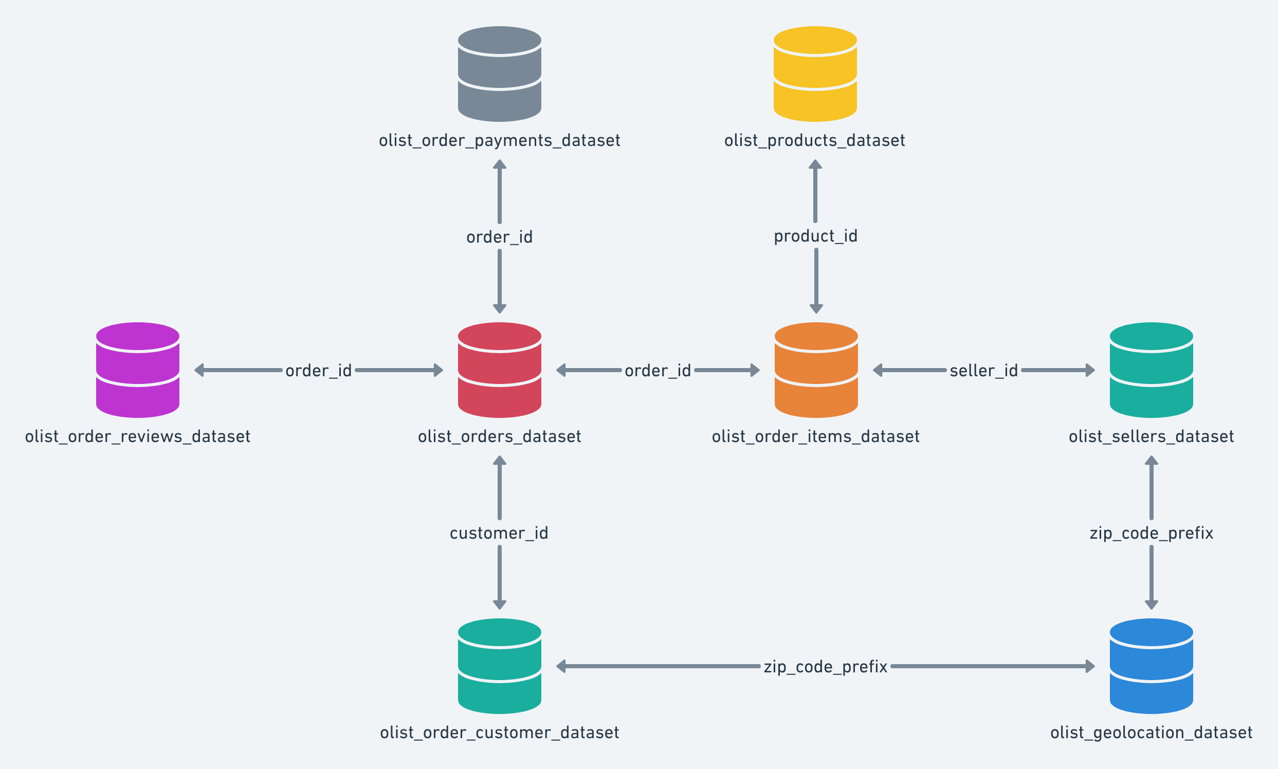
The data of Olist is divided in multiple datasets for better understanding and organization. When working with transactional data, Entity-relationship diagrams (ERD) are used for describing and defining the data models (see example below). It illustrates the logical structure of the databases.
Please refer to the following data schema when working with the Olist data. It shows with which key column we can combine the single databases. Example: To see which items are included in an order, you have to combine orders with order_items via the column order_id.
The dataset has information of 100k orders from 2016 to 2018 made at multiple marketplaces in Brazil. Its features allows viewing an order from multiple dimensions: from order status, price, payment and freight performance to customer location, product attributes and finally reviews written by customers. In addition a geolocation dataset that relates Brazilian zip codes to lat/lng coordinates is released.
This is real commercial data, it has been anonymised, and references to the companies and partners in the review text have been replaced with the names of Game of Thrones great houses.
- An order might have multiple items.
- Each item might be fulfilled by a distinct seller.
- All text identifying stores and partners where replaced by the names of Game of Thrones great houses.
The data contain the following information (excerpt):
Table orders:
| order.id | customer.id | order.status | order.purchase.timestamp | order.approved.at | order.delivered.carrier.date | order.delivered.customer.date | order.estimated.delivery.date |
|---|---|---|---|---|---|---|---|
| e481f51cbdc54678b7cc49136f2d6af7 | 9ef432eb6251297304e76186b10a928d | delivered | 2017-10-02 10:56:33 | 2017-10-02 11:07:15 | 2017-10-04 19:55:00 | 2017-10-10 21:25:13 | 2017-10-18 00:00:00 |
| … | … | … | … | … | … | … | … |
order.id: order unique identifiercustomer.id: key to the customer dataset. Each order has a unique customer.id.order.status: Reference to the order status (delivered, shipped, etc).order.purchase.timestamp: Shows the purchase timestamp.order.approved.at: Shows the payment approval timestamp.order.delivered.carrier.date: Shows the order posting timestamp. When it was handled to the logistic partner.order.delivered.customer.date: Shows the actual order delivery date to the customer.order.estimated.delivery.date: Shows the estimated delivery date that was informed to customer at the purchase moment.
Table order_items:
| order.id | order.item.id | product.id | seller.id | shipping.limit.date | price | freight.value |
|---|---|---|---|---|---|---|
| 00010242fe8c5a6d1ba2dd792cb16214 | 1 | 4244733e06e7ecb4970a6e2683c13e61 | 48436dade18ac8b2bce089ec2a041202 | 2017-09-19 09:45:35 | 58.9 | 13.3 |
| … | … | … | … | … | … | … |
order.id: order unique identifierorder.item.id: sequential number identifying number of items included in the same order.product.id: product unique identifierseller.id: seller unique identifiershipping.limit.date: Shows the seller shipping limit date for handling the order over to the logistic partner.price: item pricefreight.value: item freight value item (if an order has more than one item the freight value is splitted between items)
Table products:
| product.id | product.category.name | product.name.lenght | product.description.lenght | product.photos.qty | product.weight.g | product.length.cm | product.height.cm | product.width.cm |
|---|---|---|---|---|---|---|---|---|
| 1e9e8ef04dbcff4541ed26657ea517e5 | perfumaria | 40 | 287 | 1 | 225 | 16 | 10 | 14 |
| … | … | … | … | … | … | … | … | … |
product.id: unique product identifierproduct.category.name: root category of product, in Portuguese.product.name.lenght: number of characters extracted from the product name.product.description.lenght: number of characters extracted from the product description.product.photos.qty: number of product published photosproduct.weight.g: product weight measured in grams.product.length.cm: product length measured in centimeters.product.height.cm: product height measured in centimeters.product.width.cm: product width measured in centimeters.
Analysis
You have downloaded the data already in the last session. Let’s start by creating a script file. You can download the following template and add it to your folder 00_scripts:
---- (four dashes) at the end of a comment.As you can see the template has a couple of sections. In the following we are going to populate them step by step in order to conduct our analysis.
Session and then click Restart R1. Libraries
You can just load the tidyverse library since it attaches all the packages we will need for this analysis. For the purpose of learning, the single packages, that we need, are listed as well.
# 1.0 Load libraries ----
library(tidyverse)
# library(tibble) –> is a modern re-imagining of the data frame
# library(readr) –> provides a fast and friendly way to read rectangular data like csv
# library(dplyr) –> provides a grammar of data manipulation
# library(magrittr) –> offers a set of operators which make your code more readable (pipe operator)
# library(tidyr) –> provides a set of functions that help you get to tidy data
# library(stringr) –> provides a cohesive set of functions designed to make working with strings as easy as possible
# library(ggplot2) –> graphics
## ── Attaching packages ──────────────────────────────── tidyverse 1.3.0 ──
## ✓ ggplot2 3.3.0 ✓ purrr 0.3.4
## ✓ tibble 3.0.1 ✓ dplyr 0.8.5
## ✓ tidyr 1.0.2 ✓ stringr 1.4.0
## ✓ readr 1.3.1 ✓ forcats 0.5.0
## ── Conflicts ───────────────────────────────────────── tidyverse_conflicts() ──
## x dplyr::filter() masks stats::filter()
## x dplyr::lag() masks stats::lag()
2. Import
The files are located at /00_data/01_e-commerce/01_raw_data/. To read tha data into R we are going to use the read_csv() function from the readr package. Take a look at the help site to figure out how to use it. Also think about which data we need for our analysis. You can ignore the default arguments (the arguments which equal already a value) for now. Don’t forget to store the data into a named variable.
?read_csvWe need:
- orders (for years)
- order_items (for price)
- products (for the categories)
# 2.0 Importing Files ----
# A good convention is to use the csv file name and suffix it with tbl for the data structure tibble
order_items_tbl <- read_csv(file = "00_data/01_e-commerce/01_raw_data/olist_order_items_dataset.csv")
products_tbl    <- read_csv(file = "00_data/01_e-commerce/01_raw_data/olist_products_dataset.csv")
orders_tbl      <- read_csv(file = "00_data/01_e-commerce/01_raw_data/olist_orders_dataset.csv")
In the console you see, that read_csv() detects automatically the datatype of each column. In your environment you should see now 3 loaded tables. You can click on them to take a look at the data.
3. Examine
Use different methods to take a look and get a feel for the data.
# 3.0 Examining Data ----
# Method 1: Print it to the console
order_items_tbl
## # A tibble: 32,951 x 9
## product.id product.categor… product.name.le… product.descrip…
## <chr> <chr> <dbl> <dbl>
## 1 1e9e8ef04… perfumaria 40 287
## 2 3aa071139… artes 44 276
## 3 96bd76ec8… esporte_lazer 46 250
## 4 cef67bcfe… bebes 27 261
## 5 9dc1a7de2… utilidades_dome… 37 402
## 6 41d3672d4… instrumentos_mu… 60 745
## 7 732bd381a… cool_stuff 56 1272
## 8 2548af3e6… moveis - decora… 56 184
## 9 37cc742be… eletrodomestico… 57 163
## 10 8c9210988… brinquedos 36 1156
## # … with 32,941 more rows, and 5 more variables:
## # product.photos.qty <dbl>, product.weight.g <dbl>,
## # product.length.cm <dbl>, product.height.cm <dbl>,
## # product.width.cm <dbl>
# Method 2: Clicking on the file in the environment tab (or run View(order_items_tbl)) There you can play around with the filter.
# Method 3: glimpse() function. Especially helpful for wide data (data with many columns)
glimpse(order_items_tbl)
## Rows: 32,951
## Columns: 9
## $ product.id <chr> “1e9e8ef04dbcff4541ed26657ea517e5”, …
## $ product.category.name <chr> “perfumaria”, “artes”, “esporte_laze…
## $ product.name.lenght <dbl> 40, 44, 46, 27, 37, 60, 56, 56, 57, …
## $ product.description.lenght <dbl> 287, 276, 250, 261, 402, 745, 1272, …
## $ product.photos.qty <dbl> 1, 1, 1, 1, 4, 1, 4, 2, 1, 1, 1, 4, …
## $ product.weight.g <dbl> 225, 1000, 154, 371, 625, 200, 18350…
## $ product.length.cm <dbl> 16, 30, 18, 26, 20, 38, 70, 40, 27, …
## $ product.height.cm <dbl> 10, 18, 9, 4, 17, 5, 24, 8, 13, 10, …
## $ product.width.cm <dbl> 14, 20, 15, 26, 13, 11, 44, 40, 17, …
4. Joining data
Take a look at ?left_join(). Start by merging order_items and products and then chain all joins together.
# by automatically detecting a common column
left_join(order_items_tbl, products_tbl)
## Joining, by = "product.id"
## # A tibble: 112,650 x 15
## order.id order.item.id product.id seller.id shipping.limit.date price
## <chr> <dbl> <chr> <chr> <dttm> <dbl>
## 1 0001024… 1 4244733e0… 48436dad… 2017-09-19 09:45:35 58.9
## 2 00018f7… 1 e5f2d52b8… dd7ddc04… 2017-05-03 11:05:13 240.
## 3 000229e… 1 c777355d1… 5b51032e… 2018-01-18 14:48:30 199
## 4 00024ac… 1 7634da152… 9d7a1d34… 2018-08-15 10:10:18 13.0
## 5 00042b2… 1 ac6c36230… df560393… 2017-02-13 13:57:51 200.
## 6 00048cc… 1 ef92defde… 6426d21a… 2017-05-23 03:55:27 21.9
## 7 00054e8… 1 8d4f2bb7e… 7040e82f… 2017-12-14 12:10:31 19.9
## 8 000576f… 1 557d85097… 5996cdda… 2018-07-10 12:30:45 810
## 9 0005a1a… 1 310ae3c14… a416b6a8… 2018-03-26 18:31:29 146.
## 10 0005f50… 1 4535b0e10… ba143b05… 2018-07-06 14:10:56 54.0
## # … with 112,640 more rows, and 9 more variables: freight.value <dbl>,
## # product.category.name <chr>, product.name.lenght <dbl>,
## # product.description.lenght <dbl>, product.photos.qty <dbl>,
## # product.weight.g <dbl>, product.length.cm <dbl>,
## # product.height.cm <dbl>, product.width.cm <dbl>
# If the data had no common column name, you can provide each column name in the "by" argument. For example, by = c("a" = "b") will match x.a to y.b. The order of the columns has to match the order of the tibbles).
left_join(order_items_tbl, products_tbl, by = c("product.id" = "product.id"))
# Chaining commands with the pipe and assigning it to order_items_joined_tbl
order_items_joined_tbl <- order_items_tbl %>%
left_join(orders_tbl) %>%
left_join(products_tbl)
## Joining, by = "order.id"
## Joining, by = "product.id"
# Examine the results with glimpse()
order_items_joined_tbl %>% glimpse()
## Rows: 112,650
## Columns: 24
## $ order.id <chr> "00010242fe8c5a6d1ba2dd792cb16214…
## $ order.item.id <dbl> 1, 1, 1, 1, 1, 1, 1, 1, 1, 1, 1, …
## $ product.id <chr> "4244733e06e7ecb4970a6e2683c13e61…
## $ seller.id <chr> "48436dade18ac8b2bce089ec2a041202…
## $ shipping.limit.date <dttm> 2017-09-19 09:45:35, 2017-05-03 …
## $ price <dbl> 58.90, 239.90, 199.00, 12.99, 199…
## $ freight.value <dbl> 13.29, 19.93, 17.87, 12.79, 18.14…
## $ customer.id <chr> "3ce436f183e68e07877b285a838db11a…
## $ order.status <chr> "delivered", "delivered", "delive…
## $ order.purchase.timestamp <dttm> 2017-09-13 08:59:02, 2017-04-26 …
## $ order.approved.at <dttm> 2017-09-13 09:45:35, 2017-04-26 …
## $ order.delivered.carrier.date <dttm> 2017-09-19 18:34:16, 2017-05-04 …
## $ order.delivered.customer.date <dttm> 2017-09-20 23:43:48, 2017-05-12 …
## $ order.estimated.delivery.date <dttm> 2017-09-29, 2017-05-15, 2018-02-…
## $ product.category.name <chr> "cool_stuff", "pet_shop", "moveis…
## $ product.name.lenght <dbl> 58, 56, 59, 42, 59, 36, 52, 39, 5…
## $ product.description.lenght <dbl> 598, 239, 695, 480, 409, 558, 815…
## $ product.photos.qty <dbl> 4, 2, 2, 1, 1, 1, 1, 3, 1, 1, 1, …
## $ product.weight.g <dbl> 650, 30000, 3050, 200, 3750, 450,…
## $ product.length.cm <dbl> 28, 50, 33, 16, 35, 24, 27, 35, 3…
## $ product.height.cm <dbl> 9, 30, 13, 10, 40, 8, 5, 75, 12, …
## $ product.width.cm <dbl> 14, 40, 33, 15, 30, 15, 20, 45, 1…You should have a new variable called order_items_joined_tbl stored in your Global Environment.
5. Wrangling data
Data manipulation & Cleaning. Usually a data scientist will spend most of his/her time at this section. These are the issues we are facing for our analysis:
- Take a look at the colum
product.category.name(e.g. by runningorder_items_joined_tbl$product.category.name). Some entries seem to have a main and a sub product category separated by a-. For example there are furnitures - office (moveis - escritorio) and furnitures - kitchen_dining_laundry_garden (moveis - cozinha_area_de_servico_jantar_e_jardim). You can print all unique entires, that containmoveiswith the following code chunk:
order_items_joined_tbl %>%
  select(product.category.name) %>%
  filter(str_detect(product.category.name, "moveis")) %>%
  unique()
## # A tibble: 6 x 1
##   product.category.name
##
## 1 moveis - decoracao
## 2 moveis - escritorio
## 3 moveis - cozinha_area_de_servico_jantar_e_jardim
## 4 moveis - sala
## 5 moveis - quarto
## 6 moveis - colchao_e_estofado
We want to analyze the sales by product category. To do it by main and by sub categories we have to separate product category name in product main and sub category name.
Moreover, we want to report the freight value as revenue as well. Therefore, we have to add the total price (sales price + freight value) to the data.
To fix those issues we are going to do a series of dplyr operations on the object order_items_joined_tbl:
# 5.0 Wrangling Data ----
# All actions are chained with the pipe already. You can perform each step separately and use glimpse() or View() to validate your code. Store the result in a variable at the end of the steps.
order_items_wrangled_tbl <- order_items_joined_tbl %>%
# 5.1 Separate product category name in main and sub
separate(col = product.category.name,
into = c("main.category.name", "sub.category.name"),
sep = " - ",
# Setting remove to FALSE to keep the original column
remove = FALSE) %>%
# 5.2 Add the total price (price + freight value)
# Add a column to a tibble that uses a formula-style calculation of other columns
mutate(total.price = price + freight.value) %>%
# 5.3 Optional: Reorganize. Using select to grab or remove unnecessary columns
# 5.3.1 by exact column name
select(-shipping.limit.date, -order.approved.at) %>%
# 5.3.2 by a pattern (we don't need columns that start with "product." or end with ".date")
# You can use the select_helpers to define patterns.
# Type ?ends_with and click on Select helpers in the documentation
select(-starts_with("product.")) %>%
select(-ends_with(".date")) %>%
# 5.3.3 Actually we need the column "product.id". Let's bind it back to the data
bind_cols(order_items_joined_tbl %>% select(product.id)) %>%
# 5.3.4 You can reorder the data by selecting the columns in your desired order.
# You can use select_helpers like contains() or everything()
select(contains("timestamp"), contains(".id"),
main.category.name, sub.category.name, price, freight.value, total.price,
everything()) %>%
# 5.4 Rename columns because we actually wanted underscores instead of the dots
# (one at the time vs. multiple at once)
rename(order_date = order.purchase.timestamp) %>%
set_names(names(.) %>% str_replace_all("\\.", "_"))You will get a Warning message:
Expected 2 pieces. Missing pieces filled with `NA` in 88045 rows...You can ignore that, because it is just informing you, that some product_categories do not have a subcategory. Those entries will be filled with NA (Not available). This is exactly what we want.
Explanation of the last step:
names()returns all of the column names of a tibble as a character vector.- The dot
.is used in dplyr pipes%>%to supply the incoming data in another part of the function. The dot enables passing the incoming tibble to multiple spots in the function. str_replace_all()takes a "pattern" argument to find a pattern using Regular Expressions (RegEx) and a "replacement" argument to replace the pattern. Regex is used in programming to match strings. The period.is a special character. It needs to be "escaped" using"\\.". We will use RegEx again in the next session.
6. Business Insights
Now that we got the data in a good format, we can start to create business insights for that. We are going to do two analyses. The first is Sales by year and the second is sales by category. This will be a 2 step process for each analysis: Step 1: Manipulate / prepare the data and Step 2: Visualize it (this is one of the most important skills a data scientist needs to know).
Sales by year: Step 1
In the first step we need to do the following:
- Select the columns we need
- Extract the years from the date (we will use the lubridate library)
- Group the data by years and summarize the sales
# 6.0 Business Insights ----
# 6.1 Sales by Year ----
library(lubridate)
# Step 1 - Manipulate
revenue_by_year_tbl <- order_items_wrangled_tbl %>%
# Select columns
select(order_date, total_price) %>%
# Add year column
mutate(year = year(order_date)) %>%
# Grouping by year and summarizing sales
group_by(year) %>%
summarize(revenue = sum(total_price)) %>%
# Optional: Add a column that turns the numbers into a currency format (makes it in the plot optically more appealing)
mutate(revenue_text = scales::dollar(revenue))
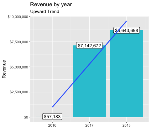
revenue_by_year_tbl
## # A tibble: 3 x 3
## year revenue revenue_text
## <dbl> <dbl> <chr>
## 1 2016 57183. $57,183
## 2 2017 7142672. $7,142,672
## 3 2018 8643698. $8,643,698Sales by year: Step 2
Now that we got the data in a good format, we can visualize it with ggplot2. A bar plot is well suited for this case. This section will give you just some exposure to visualization. Session 5 will be completely dedicated to this topic.
- Create a canvas
- Select plotting style (bar plot in this case)
- Format the plot
# 6.1 Sales by Year ----
  # Step 2 - Visualize
  revenue_by_year_tbl %>%
  # Setup canvas with the columns year (x-axis) and revenue (y-axis)
  ggplot(aes(x = year, y = revenue)) +
  # Geometries
  geom_col(fill = "#2DC6D6") + # Use geom_col for a bar plot
  geom_label(aes(label = revenue_text)) + # Adding labels to the bars
  geom_smooth(method = "lm", se = FALSE) + # Adding a trendline
  # Formatting
  scale_y_continuous(labels = scales::dollar) + # Change the y-axis
  labs(
    title    = "Revenue by year",
    subtitle = "Upward Trend",
    x = "", # Override defaults for x and y
    y = "Revenue"
  )
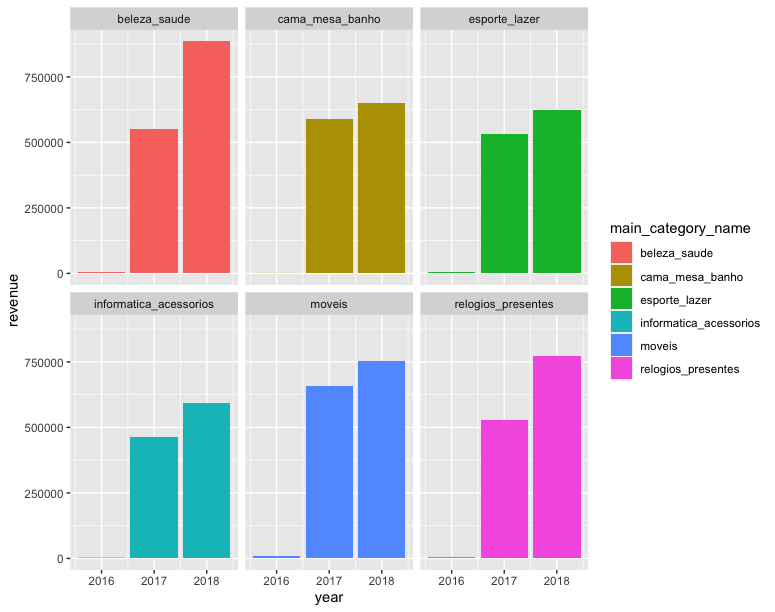
Revenue by years was a first great vizualisation. But often times, what we want to do is dive into subsets of data. Showing Revenue by year and by category is a good way to extract more details from the existing data.
Sales by category: Step 1
- Select columns
- Filter cagegories with revenue > 1.000.000 (Otherwise the plot will be confusingly packed with data)
- Group by year and category simultaneously
# 6.2 Sales by Year and Category ----
# Step 1 - Manipulate
revenue_by_year_cat_main_tbl <- order_items_wrangled_tbl %>%
# Select columns and add a year
select(order_date, total_price, main_category_name) %>%
mutate(year = year(order_date)) %>%
# Filter > 1.000.000
group_by(main_category_name) %>%
filter(sum(total_price) > 1000000) %>% # If you run the code up here, R will tell you that we have 6 groups
ungroup() %>%
# Group by and summarize year and main catgegory
group_by(year, main_category_name) %>%
summarise(revenue = sum(total_price)) %>%
ungroup() %>%
# Format $ Text
mutate(revenue_text = scales::dollar(revenue))
revenue_by_year_cat_main_tbl
## # A tibble: 18 x 4
## year main_category_name revenue revenue_text
## <dbl> <chr> <dbl> <chr>
## 1 2016 beleza_saude 5637. $5,637
## 2 2016 cama_mesa_banho 607. $607
## 3 2016 esporte_lazer 3927. $3,927
## 4 2016 informatica_acessorios 1740. $1,740
## 5 2016 moveis 8776. $8,776
## 6 2016 relogios_presentes 3468. $3,468
## 7 2017 beleza_saude 550420. $550,420
## 8 2017 cama_mesa_banho 590280. $590,280
## 9 2017 esporte_lazer 530730. $530,730
## 10 2017 informatica_acessorios 462761. $462,761
## 11 2017 moveis 659522. $659,522
## 12 2017 relogios_presentes 530087. $530,087
## 13 2018 beleza_saude 885191. $885,191
## 14 2018 cama_mesa_banho 650795. $650,795
## 15 2018 esporte_lazer 621999. $621,999
## 16 2018 informatica_acessorios 594771. $594,771
## 17 2018 moveis 752618. $752,618
## 18 2018 relogios_presentes 771987. $771,987Sales by category: Step 2
- Create a canvas
- Select plotting style (combination of a facet wrap and bar plots in this case)
# Step 2 - Visualize
revenue_by_year_cat_main_tbl %>%
  # Set up x, y, fill
  ggplot(aes(x = year, y = revenue, fill = main_category_name)) +
  # Geometries
  geom_col() + # Run up to here to get a stacked bar plot
  # Facet
  facet_wrap(~ main_category_name) +
  # Formatting
  scale_y_continuous(labels = scales::dollar) +
  labs(
    title = "Revenue by year and main category",
    subtitle = "Each product category has an upward trend",
    fill = "Main category" # Changes the legend name
  )
Checks at this Point
- Make sure that you have two plots, one for aggregated sales by year and one for sales by year and main category
- Save your work
7. Writing files
Excel is great when others may want access to your data that are Excel users. For example, many Busienss Intelligence Analysts use Excel not R. CSV is a good option when others may use different languages such as Python, Java or C++. RDS is a format used exclusively by R to save any R object in it’s native format
# 7.0 Writing Files ----
  # If you want to interact with the filesystem use the fs package
  install.packages("fs")
  library(fs)
  fs::dir_create("00_data/01_e-commerce/04_wrangled_data_student")
  # 7.1 Excel ----
  install.packages("writexl")
  library("writexl")
  order_items_wrangled_tbl %>%
    write_xlsx("00_data/01_e-commerce/04_wrangled_data_student/order_items.xlsx")
  # 7.2 CSV ----
  order_items_wrangled_tbl %>%
    write_csv("00_data/01_e-commerce/04_wrangled_data_student/order_items.csv")
  # 7.3 RDS ----
  order_items_wrangled_tbl %>%
write_rds("00_data/01_e-commerce/04_wrangled_data_student/order_items.rds")Code Checkpoint
Periodically I’ll have Code Checkpoints to to help if you get stuck on a code error or want to verify output in your data project. The Code Checkpoint contains working code up to this point.
If you run into errors, you can download the code from the closest next Code Checkpoint, run it, and compare the results to yours.
Datacamp
Challenge
Your challenges are pretty similar like the analyses we just did:
- Analyze the sales by location (state) of the sellers (bar plot). You will need to import the following table. Since
stateandcityare multiple features (variables), they should be split. Where are most of the sellers located?
Table sellers:
| seller.id | seller.zip.code.prefix | seller.location |
|---|---|---|
| 3442f8959a84dea7ee197c632cb2df15 | 13023 | campinas, SP |
| … | … | … |
seller.id: seller unique identifierseller.zip.code.prefix: first 5 digits of seller zip codeseller.location: combination of seller city name and seller state
Analyze the sales by location and year (facet_wrap). If you filter the minimum revenue by 100.000 you should get 9 groups.
Do the initial analysis again, but this time use the english translation for the categories. There is a file in the
01_raw_datafolder namedproduct_category_name_translation.xlsx. Left_join that to the other data. (If you have downloaded the data before the 16.06., please download again. There have been minor changes.)
Insert your scripts and results into your website. It might be easier to move your entire project folder into your website folder.